Chapter 2 Creating the layers
This chapter will cover the necessary steps to make layers which will be visualised in the app:
- kriging
- spatial joins
- aggregating interpolations within polygons
2.1 Kriging
Kriging is an interpolation method that we use for iTRAQI. We pass observed values with known outcomes and coordinates and use kriging to get predicted values for new coordinates (the rest of Queensland).
2.1.1 Data
First, we will download the data that we used for acute care travel time. Each row in the data has a coordinate (x,y) and outcome that we will be using for interpolation (time)
Table 2.1 and figure 2.1 show a preview of the data that we will be using.
library(tidyverse)
library(leaflet)
save_dir <- "input"
githubURL <- glue::glue("https://raw.githubusercontent.com/RWParsons/iTRAQI_app/main/input/QLD_locations_with_RSQ_times_20220718.csv")
download.file(githubURL, file.path(save_dir, "df_towns.csv"), method = "curl")
df_towns <- read.csv(file.path(save_dir, "df_towns.csv")) %>%
select(location, x, y, centre = acute_care_centre, time = acute_time)
knitr::kable(
head(df_towns, 10),
caption = "A preview of the data used for kriging",
booktabs = TRUE
)| location | x | y | centre | time |
|---|---|---|---|---|
| Boigu Island | 142.2153 | -9.260192 | Townsville University Hospital | 493 |
| Saibai Island | 142.6217 | -9.380440 | Townsville University Hospital | 491 |
| Erub (Darnley) Island | 143.7703 | -9.585443 | Townsville University Hospital | 527 |
| Yorke Island | 143.4073 | -9.750172 | Townsville University Hospital | 503 |
| Iama (Yam) Island | 142.7744 | -9.900403 | Townsville University Hospital | 466 |
| Mer (Murray) Island | 144.0504 | -9.918105 | Townsville University Hospital | 534 |
| Mabuiag Island | 142.1829 | -9.957180 | Townsville University Hospital | 449 |
| Badu Island | 142.1388 | -10.123220 | Townsville University Hospital | 440 |
| St Pauls | 142.3349 | -10.184880 | Townsville University Hospital | 436 |
| Warraber Island | 142.8238 | -10.207260 | Townsville University Hospital | 456 |
leaflet() %>%
addProviderTiles("CartoDB.VoyagerNoLabels") %>%
addCircleMarkers(
lng = df_towns$x,
lat = df_towns$y,
popup = glue::glue( # customise your popups with html tags
"<b>Location: </b>{df_towns$location}<br>",
"<b>Time to acute care (minutes): </b>{df_towns$time}"
),
radius = 2, fillOpacity = 0,
)Figure 2.1: leaflet map with locations
We will convert our data.frame into a spatial data.frame and load the gstat package as we will be using it for the kriging (gstat::krige()).
library(sp)
library(gstat)
library(sf)
coordinates(df_towns) <- ~ x + y2.1.2 Making a grid of values for interpolation
Another key ingredient to do kriging is to have a grid of coordinates for which we want predictions (QLD).
The code below achieves this by creating a grid across all coordinates of QLD and keeping only those which intersect with the QLD boundary polygon. The initial grid contains coordinates for all combinations of latitudes and longitudes in QLD (which includes a lot of water of the north east for which we don’t need interpolated values). Figure 2.2 shows the initial grid made using sp::makegrid() in blue and the intersect between this and the QLD boundary in orange. We will use the values which are within the QLD boundary for kriging.
The cellsize we use here is large to save computation time (and to highlight a problem that we will come across very soon). This controls the resolution of the interpolation - the smaller the cellsize, the greater the spatial resolution. This is in degrees units (0.1 degree = 11.1km) so only having one prediction for every 11.1km² in QLD may mean that we miss out on some valuable information! (I’ll come back to this!)
aus <- raster::getData("GADM", path = "input", country = "AUS", level = 1)
qld_boundary <- aus[aus$NAME_1 == "Queensland", ]
qld_boundary_sf <- st_as_sfc(qld_boundary)
cellsize <- 0.05
grid <- makegrid(qld_boundary, cellsize = cellsize)
pnts_sf <- st_as_sf(grid, coords = c("x1", "x2"), crs = st_crs(qld_boundary))
pnts_in_qld <- st_intersection(pnts_sf, qld_boundary_sf) %>%
st_coordinates() %>%
as.data.frame()
ggplot() +
geom_point(data = grid, aes(x1, x2), col = "blue") +
geom_point(data = pnts_in_qld, aes(X, Y), col = "orange") +
coord_equal() +
labs(
x = "Longitude",
y = "Latitude"
)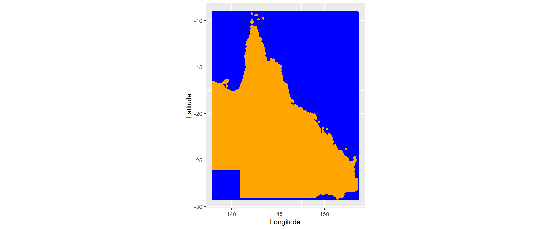
Figure 2.2: coordinates that we will use for kriging (initial grid in blue and those than intersect with QLD boundary in orange)
2.1.3 Kriging (finally)
Now we are ready to do the kriging. gstat::krige() requires that the newdata be of class Spatial, sf, or stars. Here, I specify the coordinates using sp::coordinates(). It also requires that you specify the variogram model within - here we use a circular model vgm("Cir") but there may be better choices for other data.
Figure 2.3 shows the map with the interpolated values from kriging.
lzn_vgm <- variogram(time ~ 1, df_towns)
lzn_fit <- fit.variogram(lzn_vgm, model = vgm("Sph"))
coordinates(pnts_in_qld) <- ~ X + Y
kriged_layer <-
krige(
formula = time ~ 1,
locations = df_towns,
newdata = pnts_in_qld,
model = lzn_fit
) %>%
as.data.frame()## [using ordinary kriging]ggplot(data = kriged_layer, aes(X, Y, col = var1.pred)) +
geom_point() +
scale_colour_gradientn(colors = c("yellow", "orange", "red", "black")) +
coord_equal() +
labs(
x = "Longitude",
y = "Latitude"
)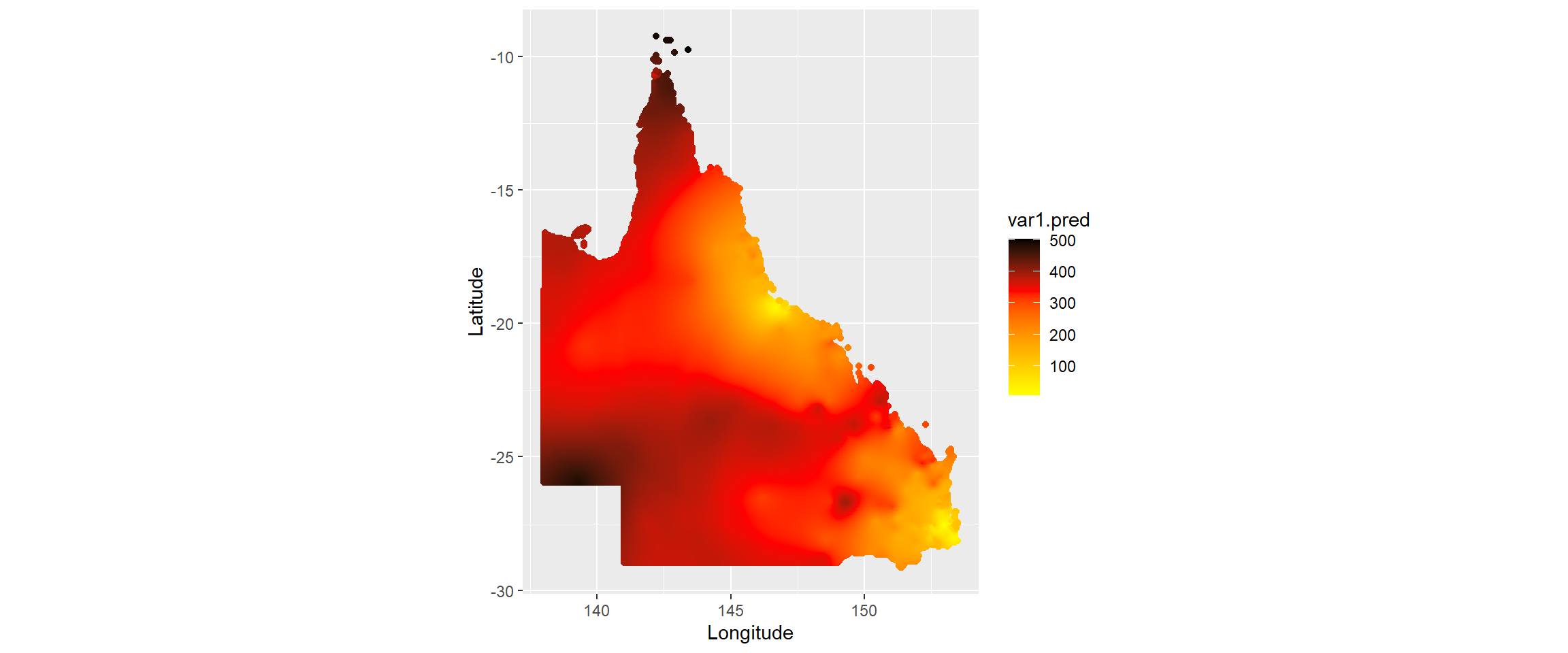
Figure 2.3: coordinates that we will use for kriging (initial grid in blue and those than intersect with QLD boundary in orange)
2.1.4 Making rasters
Now we can turn our grid of interpolated values into the rasters that we can then use in a leaflet map. We use the raster package. Figure ?? shows our kriged output as a raster on a leaflet map, the same type of objects as what’s used in iTRAQI.
raster_layer <- raster::rasterFromXYZ(kriged_layer, crs = 4326, res = 0.05)
raster_layer <- raster::raster(raster_layer, layer = 1) # layer=1 to select the prediction values rather than the variance
leaflet() %>%
addProviderTiles("CartoDB.VoyagerNoLabels") %>%
addRasterImage(x = raster_layer, colors = "YlOrRd")Figure 2.4: coordinates that we will use for kriging (initial grid in blue and those than intersect with QLD boundary in orange)
2.2 Polygons
We are going to download our polygons from the Australian Bureau of Statistics.
The link to the downloads page for the 2016 Australian Statistical Geography Standard (ASGS) files are here and the particular file that we are going to download is the ‘Queensland Mesh Blocks ASGS Ed 2016 Digital Boundaries in ESRI Shapefile Format’.
You will have to download the zipped file and unzip it somewhere locally. I’ve done so and saved it in the same directory as the other downloaded files and unzipped it into a folder there called ‘qld_shape’. Having done that, I can import it using st_read()
qld_SAs2016 <- st_read(file.path(save_dir, "qld_shape/MB_2016_QLD.shp"))## Reading layer `MB_2016_QLD' from data source
## `C:\Users\Rex\Documents\R_projects\interactive-maps\input\qld_shape\MB_2016_QLD.shp'
## using driver `ESRI Shapefile'
## replacing null geometries with empty geometries
## Simple feature collection with 69764 features and 16 fields (with 25 geometries empty)
## Geometry type: POLYGON
## Dimension: XY
## Bounding box: xmin: 137.9943 ymin: -29.1779 xmax: 153.5522 ymax: -9.142176
## Geodetic CRS: GDA94head(qld_SAs2016)## Simple feature collection with 6 features and 16 fields (with 1 geometry empty)
## Geometry type: POLYGON
## Dimension: XY
## Bounding box: xmin: 144.5488 ymin: -22.97163 xmax: 147.0728 ymax: -19.24556
## Geodetic CRS: GDA94
## MB_CODE16 MB_CAT16 SA1_MAIN16 SA1_7DIG16 SA2_MAIN16 SA2_5DIG16
## 1 30000009499 NOUSUALRESIDENCE 39999949999 3949999 399999499 39499
## 2 30000010000 Parkland 31802148912 3148912 318021489 31489
## 3 30000020000 Parkland 31802148912 3148912 318021489 31489
## 4 30000030000 Parkland 31802148912 3148912 318021489 31489
## 5 30000050000 Residential 31503140809 3140809 315031408 31408
## 6 30000160000 Residential 31503140808 3140808 315031408 31408
## SA2_NAME16 SA3_CODE16 SA3_NAME16 SA4_CODE16
## 1 No usual address (Qld) 39999 No usual address (Qld) 399
## 2 Townsville - South 31802 Townsville 318
## 3 Townsville - South 31802 Townsville 318
## 4 Townsville - South 31802 Townsville 318
## 5 Barcaldine - Blackall 31503 Outback - South 315
## 6 Barcaldine - Blackall 31503 Outback - South 315
## SA4_NAME16 GCC_CODE16 GCC_NAME16 STE_CODE16
## 1 No usual address (Qld) 39499 No usual address (Qld) 3
## 2 Townsville 3RQLD Rest of Qld 3
## 3 Townsville 3RQLD Rest of Qld 3
## 4 Townsville 3RQLD Rest of Qld 3
## 5 Queensland - Outback 3RQLD Rest of Qld 3
## 6 Queensland - Outback 3RQLD Rest of Qld 3
## STE_NAME16 AREASQKM16 geometry
## 1 Queensland 0.0000 POLYGON EMPTY
## 2 Queensland 0.0387 POLYGON ((147.0641 -19.2466...
## 3 Queensland 0.0071 POLYGON ((147.0715 -19.2576...
## 4 Queensland 0.0004 POLYGON ((147.0615 -19.2460...
## 5 Queensland 0.0432 POLYGON ((145.2406 -22.9713...
## 6 Queensland 0.2156 POLYGON ((144.5493 -22.5902...This data has polygons for every Statistical Area level 1 (SA1) in Queensland but also details the SA2, SA3, and SA4 that that area is within. If we want to only use SA1’s then we are fine to use the data here, but if we want to use these higher levels too, then we would either need (1) make a new object with dissolved boundaries within that higher level or (2) download more files from the ABS for those specific levels and filter to keep only Queensland. These files that we could use, say for SA2’s are called ‘Statistical Area Level 2 (SA2) ASGS Ed 2016 Digital Boundaries in ESRI Shapefile Format’, available at that same link.
Since it’s easy to filter, and reading this book is about learning new things (and my github repository is limited to 100mb), I’ll show you the first approach that aggregates polygons within these higher levels.
Before we make a function to aggregate within different levels, I’m going to rename the columns in the object so that they’re all named consistently - you may have noticed the unique identifier for SA1’s is called ‘SA1_MAIN16’ whereas for SA3’s it’s called ‘SA3_CODE16’. I prefer ‘CODE’.
qld_SAs2016 <-
rename(qld_SAs2016, SA1_CODE16 = SA1_MAIN16, SA2_CODE16 = SA2_MAIN16)2.2.1 Dissolving polygons to get SA2s and SA3s
The function below will dissolve the boundaries for all the polygons within the SA-level that we pick. The work here is done by rmapshaper::ms_dissolve(). I’ll use this to make separate objects for SA2s and SA3s. Since this returns back only the geometry of the polygon and the name, I’ll make the same change for my SA1s. By selecting only the code, I get the object with the code AND the geometry - unless I transform the object into a data.frame first, it will always keep the geometry.
aggregate_by_SA <- function(qld_sf, SA_number) {
sa_main <- glue::glue("SA{SA_number}_CODE16")
if (!sa_main %in% names(qld_sf)) {
return(message(sa_main, " was not found in polygon layer"))
}
message(glue::glue("----- grouping polygons within SA{SA_number} -----"))
rmapshaper::ms_dissolve(qld_sf, sa_main)
}
qld_SA2s <- aggregate_by_SA(qld_sf = qld_SAs2016, SA_number = 2)## ----- grouping polygons within SA2 -----## Registered S3 method overwritten by 'geojsonlint':
## method from
## print.location dplyrqld_SA3s <- aggregate_by_SA(qld_sf = qld_SAs2016, SA_number = 3)## ----- grouping polygons within SA3 -----qld_SA1s <- qld_SAs2016 %>% select(SA1_CODE16)
head(qld_SA1s)## Simple feature collection with 6 features and 1 field (with 1 geometry empty)
## Geometry type: POLYGON
## Dimension: XY
## Bounding box: xmin: 144.5488 ymin: -22.97163 xmax: 147.0728 ymax: -19.24556
## Geodetic CRS: GDA94
## SA1_CODE16 geometry
## 1 39999949999 POLYGON EMPTY
## 2 31802148912 POLYGON ((147.0641 -19.2466...
## 3 31802148912 POLYGON ((147.0715 -19.2576...
## 4 31802148912 POLYGON ((147.0615 -19.2460...
## 5 31503140809 POLYGON ((145.2406 -22.9713...
## 6 31503140808 POLYGON ((144.5493 -22.5902...head(qld_SA2s)## Simple feature collection with 6 features and 1 field (with 1 geometry empty)
## Geometry type: GEOMETRY
## Dimension: XY
## Bounding box: xmin: 141.4665 ymin: -25.75471 xmax: 147.2964 ymax: -12.56014
## Geodetic CRS: GDA94
## SA2_CODE16 geometry
## 1 399999499 MULTIPOLYGON EMPTY
## 2 318021489 MULTIPOLYGON (((147.0641 -1...
## 3 315031408 POLYGON ((143.6141 -22.5387...
## 4 306051166 POLYGON ((145.4269 -17.1212...
## 5 306051169 POLYGON ((145.5535 -17.1354...
## 6 315011395 MULTIPOLYGON (((141.765 -12...There are some empty geometries here, so we find (and then remove) these using st_is_empty().
qld_SA1s <- qld_SA1s[!st_is_empty(qld_SA1s), , drop = FALSE]
qld_SA2s <- qld_SA2s[!st_is_empty(qld_SA2s), , drop = FALSE]
qld_SA3s <- qld_SA3s[!st_is_empty(qld_SA3s), , drop = FALSE]Run the code to become impatient and find out how long it takes leaflet to display such a detailed polygon layer.
leaflet() %>%
addTiles() %>%
addPolygons(
data = qld_SA1s,
fillColor = "Orange",
color = "black",
weight = 1
)2.2.2 Simplifying polygons to reduce rendering time with leaflet
We need to do something about this - fortunately, we don’t need all the incredible amounts of detail in the polygons for our map, so we can simplify them using rmapshaper::ms_simplify().
Simplifying the polygons can take a few minutes but it makes the maps much faster to display.
qld_SA1s <- rmapshaper::ms_simplify(qld_SA1s, keep = 0.03)
qld_SA2s <- rmapshaper::ms_simplify(qld_SA2s, keep = 0.03)
qld_SA3s <- rmapshaper::ms_simplify(qld_SA3s, keep = 0.03)
leaflet() %>%
addTiles() %>%
addPolygons(
data = qld_SA1s,
fillColor = "yellow",
color = "black",
weight = 1,
group = "SA1"
) %>%
addPolygons(
data = qld_SA2s,
fillColor = "orange",
color = "black",
weight = 1,
group = "SA2"
) %>%
addPolygons(
data = qld_SA3s,
fillColor = "red",
color = "black",
weight = 1,
group = "SA3"
) %>%
addLayersControl(
position = "topright",
baseGroups = c("SA1", "SA2", "SA3"),
options = layersControlOptions(collapsed = FALSE)
)