circacompare

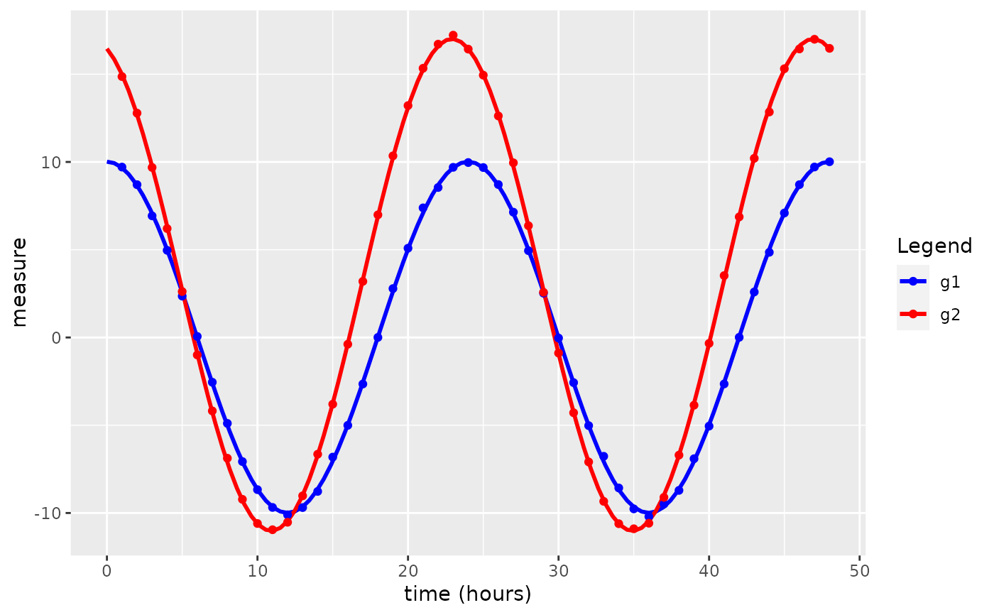
circacompare performs a comparison between two rhythmic groups of data. It tests for rhythmicity and then fits a nonlinear model with parametrization to estimate and statistically support differences in mesor, amplitude, and phase between groups.

Usage

circacompare(
  x,
  col_time,
  col_group,
  col_outcome,
  period = 24,
  alpha_threshold = 0.05,
  timeout_n = 10000,
  control = list(),
  weights = NULL,
  suppress_all = FALSE
)

Arguments

x

data.frame. This is the data.frame which contains the rhythmic data for two groups in a tidy format.

col_time

The name of the column within the data.frame, x, which contains time in hours at which the data were collected.

col_group

The name of the column within the data.frame, x, which contains the grouping variable. This should only have two levels.

col_outcome

The name of the column within the data.frame, x, which contains outcome measure of interest.

period

The period of the rhythm. For circadian rhythms, leave this as the default value, 24.

alpha_threshold

The level of alpha for which the presence of rhythmicity is considered. Default is 0.05.

timeout_n

The upper limit for the model fitting attempts. Default is 10,000.

control

list. Used to control the parameterization of the model.

weights

An optional numeric vector of (fixed) weights. When present, the objective function is weighted least squares.

suppress_all

Logical. Set to TRUE to avoid seeing errors or messages during model fitting procedure. Default is FALSE.

Value

list

Examples

df <- make_data(phi1 = 6)
out <- circacompare(
  x = df, col_time = "time", col_group = "group",
  col_outcome = "measure"
)
out
#> $plot

#> 
#> $summary
#>                                   parameter          value
#> 1  Presence of rhythmicity (p-value) for g1   7.742499e-83
#> 2  Presence of rhythmicity (p-value) for g2   9.953293e-91
#> 3                         g1 mesor estimate   1.089967e-02
#> 4                         g2 mesor estimate   2.995890e+00
#> 5                 Mesor difference estimate   2.984990e+00
#> 6              P-value for mesor difference  1.039187e-104
#> 7                     g1 amplitude estimate   1.000437e+01
#> 8                     g2 amplitude estimate   1.401390e+01
#> 9             Amplitude difference estimate   4.009528e+00
#> 10         P-value for amplitude difference  1.043910e-102
#> 11                       g1 peak time hours   2.399305e+01
#> 12                       g2 peak time hours   2.292035e+01
#> 13                Phase difference estimate  -1.072698e+00
#> 14          P-value for difference in phase   2.308806e-94
#> 15                   Shared period estimate   2.400000e+01
#> 
#> $fit
#> Nonlinear regression model
#>   model: measure ~ (k + k1 * x_group) + ((alpha + alpha1 * x_group)) *     cos((1/period) * time_r - ((phi + phi1 * x_group)))
#>    data: x
#>       k      k1   alpha  alpha1     phi    phi1 
#>  0.0109  2.9850 10.0044  4.0095 12.5646 -0.2808 
#>  residual sum-of-squares: 1.11
#> 
#> Number of iterations to convergence: 6 
#> Achieved convergence tolerance: 4.046e-08
#> 

# with sample weights (arbitrary weights for demonstration)
sw <- runif(n = nrow(df))
out2 <- circacompare(
  x = df, col_time = "time", col_group = "group",
  col_outcome = "measure", weights = sw
)
out2
#> $plot

#> 
#> $summary
#>                                   parameter          value
#> 1  Presence of rhythmicity (p-value) for g1   3.989106e-85
#> 2  Presence of rhythmicity (p-value) for g2   7.489870e-92
#> 3                         g1 mesor estimate  -1.406791e-02
#> 4                         g2 mesor estimate   2.989707e+00
#> 5                 Mesor difference estimate   3.003775e+00
#> 6              P-value for mesor difference  2.973994e-108
#> 7                     g1 amplitude estimate   1.000604e+01
#> 8                     g2 amplitude estimate   1.401206e+01
#> 9             Amplitude difference estimate   4.006026e+00
#> 10         P-value for amplitude difference  7.126206e-106
#> 11                       g1 peak time hours   2.399457e+01
#> 12                       g2 peak time hours   2.291459e+01
#> 13                Phase difference estimate  -1.079979e+00
#> 14          P-value for difference in phase   2.858438e-97
#> 15                   Shared period estimate   2.400000e+01
#> 
#> $fit
#> Nonlinear regression model
#>   model: measure ~ (k + k1 * x_group) + ((alpha + alpha1 * x_group)) *     cos((1/period) * time_r - ((phi + phi1 * x_group)))
#>    data: x
#>         k        k1     alpha    alpha1       phi      phi1 
#> -0.014068  3.003775 10.006039  4.006026 -0.001421 -0.282738 
#>  weighted residual sum-of-squares: 0.4322
#> 
#> Number of iterations to convergence: 5 
#> Achieved convergence tolerance: 3.213e-07
#>